NanoChat Speedrun, Part 1: The Code That Makes H100s Go Brrrr

Disclosure: I used AI assistance to edit and refine this post, but the ideas, interpretations, and conclusions are mine.

Read the repo alongside this. Everything below is a close reading of a specific codebase, and it will land far better if you have NanoChat open in another window. It is small enough to skim in an evening. Every claim here links to the exact file and line it came from — follow a few of them, and disagree with me where you find something I misread.

I have read a lot about transformers. Books, papers, tutorial series, the usual conference talks. Before this I would have told you I understood how they were trained.

Then in early 2026 I sat down with Andrej Karpathy’s NanoChat and read it properly — not skimmed, read — and learned more in a fortnight than I had from any of it. Not because the code is clever in a way that shows off. Because it is simple in a way that clearly took enormous effort to arrive at, and because almost every line turns out to be load-bearing once you ask why it is there.

NanoChat describes itself as a simple experimental harness for training LLMs on a single GPU node: tokenization, pretraining, fine-tuning, evaluation, inference, and a chat UI. It is small enough that a motivated reader can hold the whole thing in their head. That is the trick, and it is not an accident.

This post is the first half of a pair, and deliberately the half with no results in it. Here I read the code and write down what I expect to happen when it runs. Part 2 rents four H100s and checks.

That order matters. It is easy to explain why something was fast after watching it be fast. It is harder, and more honest, to commit to the prediction first.

One note on lineage: NanoChat’s README credits modded-nanogpt for the speedrun framing and borrows some implementation from it, but they are not the same benchmark — modded-nanogpt races to a target validation loss, while NanoChat’s speedrun spans tokenizer through chat evaluation. Ancestry, not comparison.

The shape of the repo

The executable spine is runs/speedrun.sh, and it is refreshingly literal. In order: set up the Python environment with uv, download data, train and evaluate the tokenizer, run base pretraining under torchrun, run base evaluation, download identity conversations, run SFT, run chat evaluation, generate the report.

You can read the project’s entire intent off that one file. There is no orchestration framework, no config hierarchy, no plugin system. The pipeline is a shell script because a shell script is sufficient.

That has a consequence worth stating early: the wall-clock time and the final bill do not measure raw pretraining throughput. They measure the cost of producing a usable artifact and a report about it. Those are different numbers, and the second one is the honest one.

One scope note. The reference speedrun path runs SFT and chat evaluation but not RL. NanoChat does ship scripts/chat_rl.py, but it sits outside the path I followed.

The whole project on one page

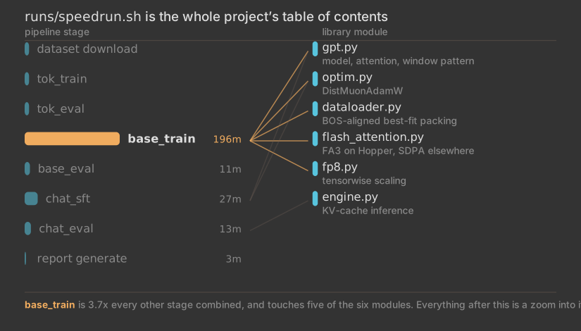
The whole project on one page. Bar length is the wall-clock time each stage actually took in my run, and the lines show which library modules each stage touches. Everything after this section is a zoom into base_train.

One integer, seven decisions

Here is the design choice that made me pay attention.

NanoChat does not ask you to tune anything to get started. The README describes a single complexity dial — the depth of the transformer — and scripts/base_train.py means it literally. From --depth, the script derives model width, attention head count, parameter count, training horizon, global batch size, learning-rate scaling, and weight decay.

The mechanism is a reference model. The d12 configuration is treated as an empirically measured anchor: its compute-optimal token horizon and batch size come from NanoChat’s own sweeps, recorded in dev/LOG.md. Every other depth is extrapolated from that anchor using scaling-law relationships plus a few hardware constraints.

The chain runs like this:

depth
  → base_dim     = depth × aspect_ratio
  → model_dim    = base_dim rounded up to a multiple of head_dim
  → num_heads    = model_dim / head_dim
  → scaling_params
  → target_tokens  = ratio × scaling_params
  → total_batch_size = B_REF × (target_tokens / D_REF)^0.383
  → learning-rate and weight-decay scaling

No single step here is exotic. What is unusual is the discipline of routing all of them through one user-facing number — and then printing the derivation so you can check it.

The rounding step shows the layering. base_dim is depth × 64, which for depth 24 gives 1536, then rounded up to a multiple of head_dim — which for 1536 does nothing. The constraint is there anyway, because attention heads must divide evenly and FA3 wants head dimensions it can tile. A depth producing an awkward width gets quietly nudged to a workable one rather than failing later inside a kernel.

The full derivation, with the paper behind each rule, is in Appendix B. The short version: batch size follows Power Lines, scaling roughly as D^0.383; learning rate follows standard square-root batch scaling; weight decay follows the T_epoch framework, keeping B / (η × λ × D) approximately constant.

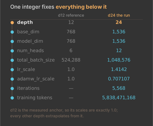
One integer fixing everything below it

One integer fixing everything below it. d12 is the measured anchor, which is why its scaling factors are exactly 1.0; the d24 column is the configuration I planned to run, derived by hand from the formulas before I ran anything.

I reproduced this derivation by hand for depth 24 before running anything, which gives Part 2 its first thing to check.

What I expect to see — Running --depth=24 should print model_dim 1536, num_heads 12, a global batch of 1,048,576 tokens, an LR scale of 1.4142, an AdamW LR scale of 0.707107, and 5,568 iterations. If any of those differ, I have misread the code.

The model it builds

The model in nanochat/gpt.py is a compact GPT-style transformer, and I am going to assume you know what that means. Rotary embeddings, RMSNorm, QK normalization, ReLU-squared MLPs, no biases, untied input and output embeddings. Individually, each of these is a choice you can find justified in a paper somewhere.

More interesting is the overall shape of the forward pass:

token embedding
  → previous-token smear
  → transformer blocks
  → optional mid-layer backout
  → final norm
  → lm_head

The two unfamiliar names are both small and cheap. The smear mixes a little of the previous token’s embedding into the current one through a learned gate — bigram-like information for almost no compute. The backout subtracts a cached mid-layer residual before the final norm, removing low-level features the output layer does not need. Neither is a headline idea. Both are the kind of thing you add after watching a lot of training curves.

--depth sets the number of repeated Block modules, and the rest of the model shape follows from the cascade above. The parameter-by-parameter breakdown is in Appendix A.

The window pattern, and the one thing the comments get wrong

The detail I did not expect is in sliding-window attention.

NanoChat tiles a pattern string across layers. The default is SSSL, where L is full context and S is shorter. Reading _compute_window_sizes:

short_window = -(-long_window // 4 // 128) * 128  # ceil to FA3 tile size

At sequence_len = 2048 that is 512 — a quarter of the context, rounded to a tile boundary. So with SSSL tiled across 24 layers, layers 3, 7, 11, 15, 19 and 23 get full context, and the other eighteen see 512 tokens.

Eighteen of twenty-four layers never look further back than a quarter of the sequence. Six layers carry every long-range interaction in the model. That is a far more aggressive bet than the phrase “sliding-window attention” suggests, and a large part of why the model is cheap to train.

A final safety line, window_sizes[-1] = (long_window, 0), forces the last layer to full context whatever the pattern says. For SSSL at depth 24 it changes nothing — layer 23 is already L. It only bites on a pattern ending in S.

This is also the one place I found where the repository contradicts itself. The --window-pattern help text in base_train.py describes S as “half context”, and the inline comment on the line above says 2048 -> 768. The arithmetic gives 512, a quarter. The docstring one line further up says “quarter context” and is correct.

The code is right and the comment is stale. In a repository built this carefully, that was genuinely the only inconsistency I found worth reporting — and it is a comment, not behaviour. Trust the arithmetic.

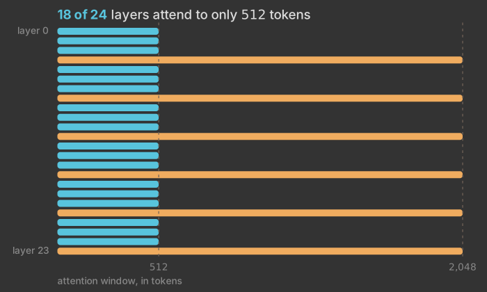
Bar width is the attention window, so the ratio is the whole story

Bar width is the attention window, so the ratio is the whole story. Eighteen of twenty-four layers never see more than 512 tokens; the six gold bars carry every long-range interaction in the model.

Why it should be fast

Everything above is design. This section is what I actually came for: the specific machinery that should keep expensive GPUs busy.

There are five mechanisms, and they are worth naming up front rather than scattering:

Fixed shapes and honest batch math — so the compiler can specialize and the global batch never drifts.
Attention — FA3 on Hopper, and nothing pretending to be FA3 elsewhere.
Precision — FP8 where it is safe, and an explicit refusal where it is not.
Communication — the optimizer owns synchronization instead of the model wrapper.
The data feeder — dense, fixed-shape batches with no padding at all.

That order runs from inside the model outward: shapes, then kernels, then numerics, then across GPUs, then the pipe feeding it all.

Fixed shapes and honest batch math

The compile call is one line and it sets the tone:

model = torch.compile(model, dynamic=False)

dynamic=False promises the compiler these shapes will not change, so it can specialize hard rather than emit code that handles anything. That is only a safe promise if the rest of the system genuinely never changes shape — which is why the dataloader later goes to such lengths to produce exactly-full rows.

The batch arithmetic is equally direct:

tokens_per_fwdbwd = args.device_batch_size * args.max_seq_len
world_tokens_per_fwdbwd = tokens_per_fwdbwd * ddp_world_size
assert total_batch_size % world_tokens_per_fwdbwd == 0

That assert does more work than it looks. total_batch_size is a property of the experiment — it comes out of the depth cascade and shapes the learning dynamics. device_batch_size is a property of the machine: however much fits in memory. Forcing the two to reconcile through gradient accumulation is what stops the effective batch quietly becoming whatever the hardware allowed.

So GPU count becomes an execution detail rather than a hyperparameter. Run the same configuration on four GPUs instead of eight and you get twice the accumulation steps and an identical global batch. The model does not know how many GPUs it trained on. (In the same spirit, the script takes manual control of Python’s garbage collector after the first step — the mark of someone who profiled their training loop and found GC pauses in it.)

What I expect to see — On four H100s with device_batch_size=16 and max_seq_len=2048, that is 32,768 tokens per rank per micro-batch and 131,072 across four ranks. To reach a 1,048,576-token global batch the script must choose exactly 8 gradient accumulation steps, and should say so.

Attention: FA3, and only on Hopper

nanochat/flash_attention.py tries to load Flash Attention 3, but only on Hopper-class GPUs, and falls back to PyTorch’s SDPA everywhere else behind an API-compatible shim.

What I like is the honesty of the fallback. It is not sold as equivalent. The training script warns that it is meaningfully less efficient, and warns harder if you combine it with sliding windows — a sliding-window mask through the generic path is expensive exactly where FA3 would be cheap. If you are not on Hopper, the advice is to stop pretending and use --window-pattern=L. Hardware-specific paths are labelled as such rather than hidden behind an abstraction that silently underperforms.

What I expect to see — On H100s the run should announce that FA3 is active. If it announces the SDPA fallback instead, every performance number afterwards is measuring something else.

Precision: what FP8 refuses to touch

FP8 is where I expected to find hand-waving, and did not.

base_train.py exposes --fp8, and on CUDA it walks the model converting eligible nn.Linear modules. nanochat/fp8.py is deliberately small: tensorwise dynamic scaling, quantize, torch._scaled_mm, dequantize. Weights use float8_e4m3fn, gradients float8_e5m2 — trading mantissa bits for range, because gradients need the range more.

The interesting word is eligible. The filter skips layers whose dimensions are not divisible by 16, and skips very small layers entirely. Neither rule is arbitrary: FP8 tensor-core paths have alignment requirements, and for a tiny matrix the quantize/dequantize overhead costs more than the faster multiply saves. dev/LOG.md adds that tensorwise scaling beat rowwise at this scale, and that the filtering was needed for stability. This is not a switch flipped because it was available.

So I counted the modules by hand. A depth-24 model has 24 blocks, each with 6 linear matrices, plus the lm_head: 145 conversions. The layers that should fail the filter are the twelve ve_gate projections, each Linear(12, 12) — 12 is not divisible by 16 — and the single smear_gate, which is Linear(24, 1) and far below any sensible minimum. That is 13 skipped, 158 total.

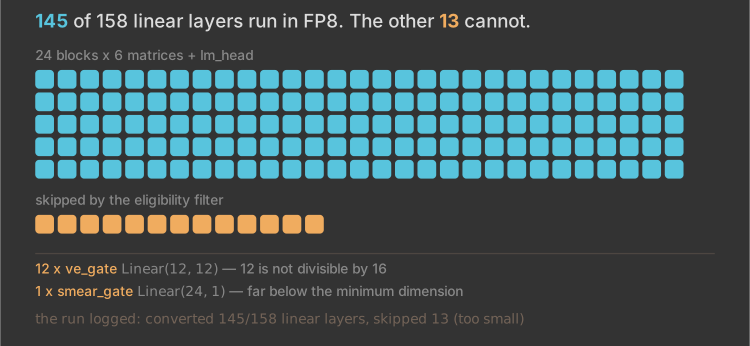
Every linear layer in the model, drawn at the same size so the proportion is honest

Every linear layer in the model, drawn at the same size so the proportion is honest. The thirteen the filter refuses are not an oversight: twelve ve_gate projections that fail the divisible-by-16 rule, and one smear_gate far below any workable dimension.

What I expect to see — The run should report converting exactly 145 of 158 linear layers and skipping 13. If the numbers differ, my reading of the filter is wrong.

Communication: the optimizer owns it

This is the part of NanoChat I would most want to show someone learning distributed training.

The model is never wrapped in PyTorch’s DistributedDataParallel. Instead, GPT.setup_optimizer() switches to DistMuonAdamW from nanochat/optim.py when the world size exceeds one, and that optimizer does the synchronization itself.

It is a hybrid: AdamW for embeddings, the unembedding and scalar-ish parameters, Muon for the matrix parameters that make up the bulk of the model. The distributed step has three explicit phases:

launch async reductions
  → wait, compute local updates, launch gathers
  → wait for gathers, copy updated parameters back

Each rank receives one slice of the gradient via reduce_scatter, updates only that slice, then all_gathers to rebuild the full parameter. Optimizer state is sharded across ranks — ZeRO-2 in style — so no rank holds a full copy of the Adam moments. For Muon parameters the code goes further, grouping tensors by shape so many small ones move as a few large ones.

Three goals, all visible in the structure: overlap communication with computation, cut optimizer memory, batch small transfers into fewer large ones. And because it is an explicit phase rather than a hook buried in a wrapper’s backward pass, you can see where the distributed boundary is. Gradients stay rank-local through all eight micro-batches — precisely where a DDP-wrapped model would already be all-reducing.

One step, four ranks, one time axis

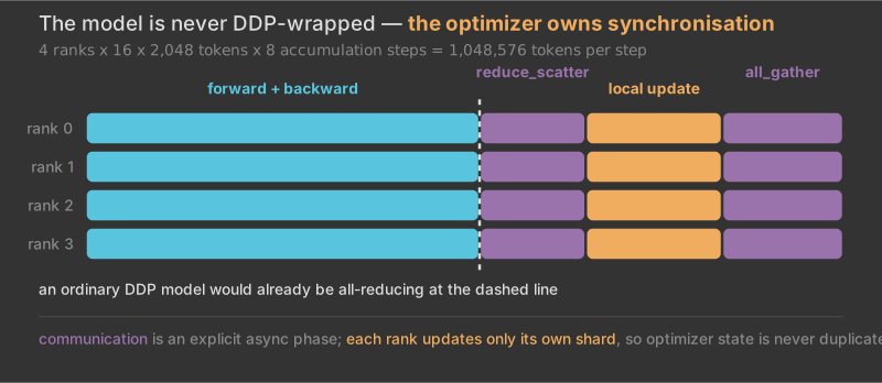
One step, four ranks, one time axis. The dashed line marks where an ordinary DDP-wrapped model would already have been all-reducing; here the gradients are still rank-local, and communication happens afterwards as an explicit async phase.

Not tested here — I can read the design, but I have no profiler trace. I will not claim communication was actually hidden behind computation, only that the code is structured so it could be.

Feeding the GPUs

Fast kernels are useless if the data pipe stalls, and this is the part of the repo I ended up admiring most.

Training data is ClimbMix parquet shards. speedrun.sh grabs 8 first so tokenizer training can start, then downloads the remaining 170 in the background while tokenizer work proceeds — even the download is pipelined. dev/LOG.md calls the switch from FineWeb-EDU to ClimbMix the single biggest improvement to the speedrun time, 2h46m down to 2h01m, and enough of a gain to move the target from d26 to d24. That is the repository’s measurement, not mine.

The runtime loader in nanochat/dataloader.py uses BOS-aligned best-fit packing. Every row begins with a BOS token. The inner loop is:

From the buffered documents, take the largest that fits entirely in the remaining space.
Repeat until nothing fits.
When nothing fits, crop the shortest buffered document to fill the remainder exactly.

Two details are easy to miss. Row capacity is T + 1 = 2049, not 2048, because inputs and targets are the same row offset by one. And the document chosen for cropping is the shortest available, not an arbitrary one, which minimizes what is discarded at that step.

The result is 100% utilization. No padding, ever. Every token in every batch is a real token contributing to the loss.

Successive states of a single row

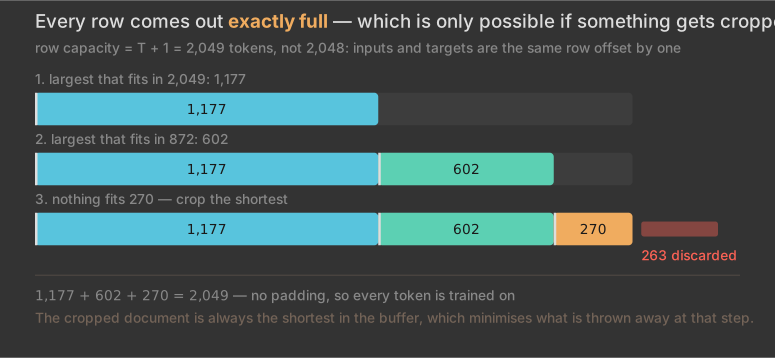
Successive states of a single row. Two documents are placed whole, then nothing in the buffer fits the remaining 270 tokens, so the shortest buffered document is cropped to fill it exactly. The red block is what that costs.

Why a third of the tokens get thrown away

dev/LOG.md records the cost: BestFit-Crop achieves 100% utilization with roughly 34.6% crop waste at T=2048. That number bothered me. A third of the corpus discarded seemed like a lot for a scheme described as best-fit.

Then I traced where it has to come from.

A document longer than row_capacity can never be selected by the best-fit search, because that search only considers documents that fit entirely in the remaining space. So the only way such a document ever leaves the buffer is the crop path — and the crop path deliberately picks the shortest buffered document. An over-long document therefore has to wait until it is the shortest thing in the buffer, which for a genuinely long document is close to never.

Over-long documents accumulate. The steady-state buffer becomes far more long-tailed than the raw corpus, and the crop rate climbs toward an equilibrium well above anything you would estimate from the document-length distribution alone.

Once you see that, the number stops looking like inefficiency. The 34.6% is not the packer doing a bad job. It is the price of insisting that every row starts at a real document boundary while T stays fixed — paid deliberately, so that every training row is dense, fixed-shape, and free of padding tokens the model would otherwise have to learn to ignore.

SFT makes the opposite trade. scripts/chat_sft.py uses the same packing, but when no conversation fits it pads the row and masks the padding out of the loss. Web text is abundant and interchangeable, so cropping it is cheap; conversations are scarce and structured, and discarding their tails would not be.

What I expect to see — Because every row is filled exactly and nothing is padded, total tokens trained should be exactly iterations × global batch, with no remainder. For 5,568 iterations at 1,048,576 tokens that is 5,838,471,168 — and the run should report that number precisely, not approximately.

Not tested here — The 34.6% figure is the repository’s measurement on real ClimbMix documents. I reproduced the accumulation trend in a small simulation, but did not instrument the actual loader. The prefetching around the loader is code structure, not a measured overlap.

After pretraining

Base pretraining dominates the cost, but it is not the whole pipeline, and the later stages are what turn a checkpoint into something you can talk to.

speedrun.sh downloads a set of synthetic identity conversations, runs scripts/chat_sft.py, then runs chat evaluation. SFT loads the base checkpoint, inherits most hyperparameters from its metadata rather than making you restate them, and reuses the same optimizer setup. The data mixture is SmolTalk, the identity conversations, MMLU, GSM8K, SimpleSpelling, and SpellingBee.

RL exists — scripts/chat_rl.py is a GRPO/REINFORCE-style loop on GSM8K — but it is deliberately simple, with no separate critic or reference-policy copies, and sits outside the speedrun path.

Success for the speedrun is measured as CORE for the base model and ChatCORE after SFT. The target is GPT-2-grade capability: a modest bar by 2026 standards, and a reasonable one for a run meant to cost less than a nice dinner.

What I expect to see

Reading code and predicting behaviour are different activities, and only the second can be wrong in a way you can check. So here is the list I wrote down before renting anything.

#	What I expect	How it would be falsified
1	`--depth=24` derives `model_dim 1536`, `num_heads 12`, batch `1,048,576`, LR scale `1.4142`, AdamW LR scale `0.707107`, `5,568` iterations	Any value differs from my hand derivation
2	Four GPUs gives `8` gradient accumulation steps and the same `1,048,576`-token global batch that eight would	The effective batch changes with GPU count
3	FP8 converts exactly `145` of `158` linear layers, skipping `13`	A different count, or different layers
4	Total tokens trained is exactly `5,568 × 1,048,576 = 5,838,471,168`	Any remainder, which would mean padding somewhere
5	FA3 activates on H100 and says so	The run falls back to SDPA
6	Base training is GPU-bound, so half the GPUs should take roughly twice as long as the 8×H100 reference of 1.65 h	Materially better or worse than about 2×
7	Utilization is high and stable — not a good average hiding a bad distribution	MFU that sags, spikes, or decays across the run
8	The whole thing lands well under the old $100 GPT-2 line	It does not

The first five are checkable from the run log alone. The last three need the run to finish.

If most of these hold, the interesting claim is not “NanoChat is fast.” It is that a codebase simple enough to read in an afternoon can be this specific about what it is doing, and be right.

What I am not testing

A list of confirmed predictions is only worth something if the scope is honest.

I am not validating the scaling-law choices. I reproduced the derivation and can confirm the code implements what it claims, but whether D^0.383 is the right exponent, or 12 the right token-to-parameter ratio, would need sweeps I have not run.

I am not attributing performance to individual components. If the run hits high utilization, that is the whole stack — model, attention, precision, optimizer, loader, compiler, hardware. Isolating any one needs ablations, and I have none.

I am not measuring kernel-level behaviour: no profiler traces, so no claims about communication actually overlapping computation. And I am not evaluating tokenizer quality, KV-cache internals, or CORE methodology. Real topics, not this post.

Part 2 rents the GPUs and works down the list.

Appendix A — Model configuration

Model piece	Parameter / default	What it affects
Context length	`sequence_len`, default `2048` via `--max-seq-len`	Maximum training context and rotary cache sizing
Vocabulary	`vocab_size`, from the tokenizer	Embedding table and `lm_head`; padded internally for efficiency
Number of blocks	`n_layer = depth`	How many transformer blocks are stacked
Width	`n_embd = model_dim`	Residual-stream width, MLP and attention matrix sizes
Query heads	`n_head = num_heads`	Number of query attention heads
KV heads	`n_kv_head`, equal to `n_head` in base training	GQA is supported in the model definition; base training does not use it
Window pattern	`window_pattern`, default `SSSL`	Per-layer attention window; `S` is a quarter of context, `L` is full

Source: GPTConfig and build_model_meta.

Appendix B — The `--depth` derivation

Inputs and reference constants:

Name	Default	Meaning
`depth`	`20`	The one knob
`aspect_ratio`	`64`	Width per layer
`head_dim`	`128`	Target attention head dimension
`target_param_data_ratio`	`12`	Tokens per parameter; the CLI help notes Chinchilla uses 20
`weight_decay`	`0.28`	Reference weight decay, before scaling
`d12_ref`	`build_model_meta(12)`	The measured anchor model
`B_REF`	`2**19` = `524,288`	Reference batch size for `d12`

Derived values:

Name	Formula	Basis
`base_dim`	`depth × aspect_ratio`	Architecture convention
`model_dim`	`ceil(base_dim / head_dim) × head_dim`	Head divisibility and FA3 tiling
`num_heads`	`model_dim / head_dim`	Follows from the above
`scaling_params`	transformer matrices + `lm_head`	Scaling Laws; `dev/LOG.md` notes this subset gave cleaner sweeps
`target_tokens`	`target_param_data_ratio × scaling_params`	Chinchilla-style token budgeting
`D_REF`	the same rule applied to `d12_ref`	The anchor’s horizon
`total_batch_size`	`B_REF × (target_tokens / D_REF)^0.383`, rounded to a power of two	Power Lines
`batch_lr_scale`	`η ∝ √(total_batch_size / B_REF)`	Square-root batch scaling for AdamW, applied to Muon as a practical assumption
`weight_decay_scaled`	`λ = λ_ref × √(B / B_REF) × (D_REF / D)`	T_epoch: keep `B / (η × λ × D)` roughly constant

Reference-model extrapolation follows muP-style transfer from the measured d12 anchor.

References

Andrej Karpathy, NanoChat.
Keller Jordan, modded-nanogpt.
Kaplan et al., Scaling Laws for Neural Language Models.
Hoffmann et al., Training Compute-Optimal Large Language Models (Chinchilla).
Yang et al., Tensor Programs V: Tuning Large Neural Networks via Zero-Shot Hyperparameter Transfer (muP).
Power Lines: Scaling Laws for Optimal Batch Size.
The T_epoch framework.
Horace He, Making Deep Learning Go Brrrr From First Principles — the source of this post’s title phrasing.